WRFChem¶

WRFChem is numerical weather prediction model coupled with chemistry.

For more information on running WRFChem, see WRFotron.

Simple plot¶

import salem
import matplotlib.pyplot as plt
import matplotlib.gridspec as gridspec
import cartopy.crs as ccrs

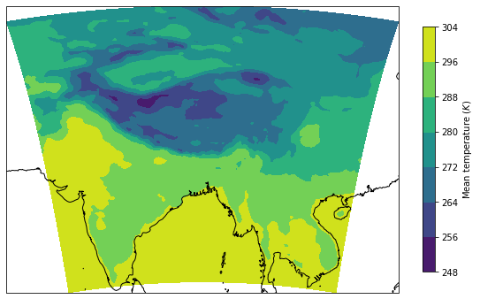
lon = ds.lon.values
lat = ds.lat.values

fig = plt.figure(1, figsize=(8, 8))
gs = gridspec.GridSpec(1, 1)

ax = fig.add_subplot(gs[0], projection=ccrs.PlateCarree())
ax.coastlines()
im = ax.contourf(lon, lat, temp_mean, transform=ccrs.PlateCarree())
fig.colorbar(im, label='Mean temperature ($K$)', shrink=0.5)

plt.tight_layout()
plt.show()

Problem: Crop arrays to shapefiles¶

Solution 1¶

Customisable cropping
Destaggered/rectilinear grid e.g. after using pp_concat_regrid.py on WRFChem output with Salem to destagger and XEMSF to regrid to rectilinear grid
- For conservative regridding, consider xgcm.

import numpy as np
import xarray as xr
import geopandas as gpd
from rasterio import features
from affine import Affine

def transform_from_latlon(lat, lon):
    """ input 1D array of lat / lon and output an Affine transformation """
    lat = np.asarray(lat)
    lon = np.asarray(lon)
    trans = Affine.translation(lon[0], lat[0])
    scale = Affine.scale(lon[1] - lon[0], lat[1] - lat[0])
    return trans * scale


def rasterize(shapes, coords, latitude='latitude', longitude='longitude', fill=np.nan, **kwargs):
    """
    Description:    
        Rasterize a list of (geometry, fill_value) tuples onto the given
        xarray coordinates. This only works for 1D latitude and longitude
        arrays.
    Usage:
        1. read shapefile to geopandas.GeoDataFrame
               `states = gpd.read_file(shp_dir+shp_file)`
        2. encode the different shapefiles that capture those lat-lons as different
           numbers i.e. 0.0, 1.0 ... and otherwise np.nan
              `shapes = (zip(states.geometry, range(len(states))))`
        3. Assign this to a new coord in your original xarray.DataArray
              `ds['states'] = rasterize(shapes, ds.coords, longitude='X', latitude='Y')`
    Arguments:
        **kwargs (dict): passed to `rasterio.rasterize` function.
    Attributes:
        transform (affine.Affine): how to translate from latlon to ...?
        raster (numpy.ndarray): use rasterio.features.rasterize fill the values
                                outside the .shp file with np.nan
        spatial_coords (dict): dictionary of {"X":xr.DataArray, "Y":xr.DataArray()}
                               with "X", "Y" as keys, and xr.DataArray as values
    Returns:
        (xr.DataArray): DataArray with `values` of nan for points outside shapefile
                        and coords `Y` = latitude, 'X' = longitude.
    """
    transform = transform_from_latlon(coords[latitude], coords[longitude])
    out_shape = (len(coords[latitude]), len(coords[longitude]))
    raster = features.rasterize(
        shapes, 
        out_shape=out_shape,
        fill=fill,
        transform=transform,
        dtype=float, 
        **kwargs
    )
    spatial_coords = {latitude: coords[latitude], longitude: coords[longitude]}
    return xr.DataArray(raster, coords=spatial_coords, dims=(latitude, longitude))

# single multipolygon
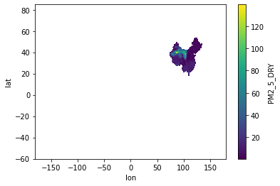
shapefile = gpd.read_file('/nfs/a68/earlacoa/shapefiles/china/CHN_adm0.shp')
shapes = [(shape, index) for index, shape in enumerate(shapefile.geometry)]

# using regridded file (xemsf)
ds = xr.open_dataset(
    '/nfs/b0122/Users/earlacoa/shared/nadia/wrfout_d01_global_0.25deg_2015-06_PM2_5_DRY_nadia.nc'
)['PM2_5_DRY'].mean(dim='time')

# apply shapefile to geometry, default: inside shapefile == 0, outside shapefile == np.nan
ds['shapefile'] = rasterize(shapes, ds.coords, longitude='lon', latitude='lat') 

# change to more intuitive labelling of 1 for inside shapefile and np.nan for outside shapefile
# if condition preserve (outside shapefile, as inside defaults to 0), otherwise (1, to mark in shapefile)
ds['shapefile'] = ds.shapefile.where(cond=ds.shapefile!=0, other=1) 

# example: crop to shapefile
# if condition (inside shapefile) preserve, otherwise (outside shapefile) remove
ds = ds.where(cond=ds.shapefile==1, other=np.nan) # could scale instead with other=ds*scale

ds.plot()

<matplotlib.collections.QuadMesh at 0x7f3bb67d42b0>

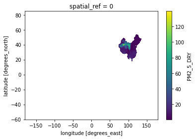
Solution 2¶

Cropping only
Destaggered/rectilinear grid e.g. after using pp_concat_regrid.py on WRFChem output with Salem to destagger and XEMSF to regrid to rectilinear grid
- For conservative regridding, consider xgcm.

import xarray as xr
import geopandas as gpd
import rioxarray
from shapely.geometry import mapping

shapefile = gpd.read_file('/nfs/a68/earlacoa/shapefiles/china/CHN_adm0.shp', crs="epsg:4326")

ds = xr.open_dataset(
    '/nfs/b0122/Users/earlacoa/shared/nadia/wrfout_d01_global_0.25deg_2015-06_PM2_5_DRY_nadia.nc'
)['PM2_5_DRY'].mean(dim='time')

ds.rio.set_spatial_dims(x_dim="lon", y_dim="lat", inplace=True)
ds.rio.write_crs("epsg:4326", inplace=True)
ds_clipped = ds.rio.clip(shapefile.geometry.apply(mapping), shapefile.crs, drop=False)

ds_clipped.plot()

<matplotlib.collections.QuadMesh at 0x7f3bbc9ee280>

Solution 3¶

Staggered grid
- WRFChem projection is normally on a Arakawa-C Grid
- e.g. intermediate WRFChem files that need to be reused (wrfiobiochemi)
- e.g. raw wrfout file (after postprocessing) still on Arakawa-C Grid (2D lat/lon coordinates)

import numpy as np
import xarray as xr
import pandas as pd
import geopandas as gpd # ensure version > 0.8.0

# WARNING: the double for loop of geometry creation and checking is very slow
# the mask in the cell below has already been calculated
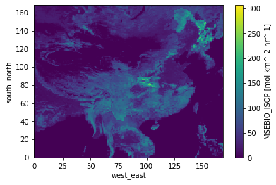
ds = xr.open_dataset('/nfs/b0122/Users/earlacoa/shared/nadia/wrfbiochemi')['MSEBIO_ISOP']
shapefile = gpd.read_file('/nfs/a68/earlacoa/shapefiles/china/CHN_adm0.shp')
mask = np.empty([ds.south_north.shape[0], ds.west_east.shape[0]])
mask[:] = np.nan

for index_lat in range(ds.south_north.shape[0]):
    for index_lon in range(ds.west_east.shape[0]):
        lat = ds.isel(south_north=index_lat).isel(west_east=index_lon).XLAT.values[0]
        lon = ds.isel(south_north=index_lat).isel(west_east=index_lon).XLONG.values[0]

        point_df = pd.DataFrame({'longitude': [lon], 'latitude': [lat]})
        point_geometry = gpd.points_from_xy(point_df.longitude, point_df.latitude, crs="EPSG:4326")
        point_gdf = gpd.GeoDataFrame(point_df, geometry=point_geometry)

        point_within_shapefile = point_gdf.within(shapefile)[0]
        
        if point_within_shapefile:
            mask[index_lat][index_lon] = True

# bring in mask which computed earlier
ds = xr.open_dataset('/nfs/b0122/Users/earlacoa/shared/nadia/wrfbiochemi')
mask = np.load('/nfs/b0122/Users/earlacoa/shared/nadia/mask_china.npz')['mask']

# demo - removing values in mask
demo = ds['MSEBIO_ISOP'].where(cond=mask!=True, other=np.nan)
demo.plot()

<matplotlib.collections.QuadMesh at 0x7f3bb4be2790>

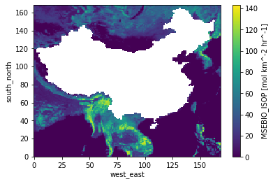
# example - doubling isoprene emissions within mask
ds['MSEBIO_ISOP'] = ds['MSEBIO_ISOP'].where(cond=mask!=True, other=2*ds['MSEBIO_ISOP'])
ds['MSEBIO_ISOP'].plot()

<matplotlib.collections.QuadMesh at 0x7f3bbcd0bbe0>

# saving back into dataset
ds.to_netcdf('/nfs/b0122/Users/earlacoa/shared/nadia/wrfbiochemi_double_isoprene_china')

# check that doubling persisted
ds_original = xr.open_dataset('/nfs/b0122/Users/earlacoa/shared/nadia/wrfbiochemi')['MSEBIO_ISOP']
ds_double = xr.open_dataset('/nfs/b0122/Users/earlacoa/shared/nadia/wrfbiochemi_double_isoprene_china')['MSEBIO_ISOP']

fraction = ds_double / ds_original

print(fraction.max().values)
print(fraction.min().values)
print(fraction.mean().values)

0
0
4608158