Tips to speed up Python¶

Contents¶

Hang on, don’t optimise too early¶

Trade-offs e.g. complexity, speed, memory, disk, readability, time, effort, etc.
- Check that code is correct (tested, documented).
- Is optimisation needed?
- If yes, optimise code and data.
- If more needed, parallelise.

Plot idea from Dask-ML.

How fast is it?¶

Profiling (i.e. find the bottlenecks)
- Speed
  - IPython magic (Jupyter Lab)
    - Line: %timeit
    - Cell: %%timeit
    - If pip install line_profiler:
      - First load module: %load_ext line_profiler
      - Scripts: %prun
      - Line-by-line: %lprun
        
        @profile decorator around the function
- Memory
  - If pip install memory_profiler:
  - First load module:
    - %load_ext memory_profiler
    - Line: %memit
    - Cell: %%memit
    - Line-by-line: %mprun
Profile parallel code

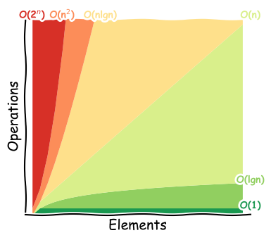
How fast could it go?¶

Time-space complexity
- Big O notation where O is the order of operations, O(…).
- Ignores constants and takes the largest order, so O(2n² + 3n) would be O(n²).
- Important for large number of elements, N.
- Typical case.
- Constant time means per machine operation.

Plot idea from Big O Cheat Sheet

Potential improvements¶

Append to lists, rather than concatenating¶

Lists are allocated twice the memory required, so appending fills this up in O(1) (long-term average), while concatenating creates a new list each time in O(n).

%%timeit
my_list = []
for num in range(1_000):
    my_list += [num] # time O(n)

46.5 µs ± 76.3 ns per loop (mean ± std. dev. of 7 runs, 10000 loops each)

%%timeit
my_list = []
for num in range(1_000):
    my_list.append(num) # time O(1)

35.6 µs ± 130 ns per loop (mean ± std. dev. of 7 runs, 10000 loops each)

Move loop-invariants outside loops¶

%%timeit
for num in range(1_000_000):
    constant = 500_000
    bigger_num = max(num, constant)

124 ms ± 462 µs per loop (mean ± std. dev. of 7 runs, 10 loops each)

%%timeit
constant = 500_000
for num in range(1_000_000):
    bigger_num = max(num, constant)

115 ms ± 196 µs per loop (mean ± std. dev. of 7 runs, 10 loops each)

Use built-in functions ¶

Optimised in C (statically typed and compiled).

nums = [num for num in range(1_000_000)]

%%timeit
count = 0
for num in nums: # time O(n)
    count += 1

23.8 ms ± 920 µs per loop (mean ± std. dev. of 7 runs, 10 loops each)

%timeit len(nums) # time O(1)

42.7 ns ± 2.1 ns per loop (mean ± std. dev. of 7 runs, 10000000 loops each)

Use optimal data types ¶

Common and additional data structures.
- e.g. dictionaries are fast to search, O(1).

Example from Luciano Ramalho, Fluent Python, Clear, Concise, and Effective Programming, 2015. O’Reilly Media, Inc.

haystack_list = np.random.uniform(low=0, high=100, size=(1_000_000))

haystack_dict = {key: value for key, value in enumerate(haystack_list)}

needles = [0.1, 50.1, 99.1]

%%timeit
needles_found = 0
for needle in needles:
    if needle in haystack_list: # time O(n) within list
        needles_found += 1

602 µs ± 13.5 µs per loop (mean ± std. dev. of 7 runs, 1000 loops each)

%%timeit
needles_found = 0
for needle in needles:
    if needle in haystack_dict: # time O(1) within dict
        needles_found += 1

138 ns ± 0.213 ns per loop (mean ± std. dev. of 7 runs, 10000000 loops each)

Many more examples e.g.:
- Generators save memory by yielding only the next iteration.
- Memory usage for floats/integers of 16 bit < 32 bit < 64 bit.
- For NetCDFs, using engine='h5netcdf' with xarray can be faster, over than the default engine='netcdf4'.
- Compression: If arrays are mostly 0, then can save memory using sparse arrays.
- Chunking: If need all data, then can load/process in chunks to reduce amount in memory: Zarr for arrays, Pandas.
- Indexing: If need a subset of the data, then can index (multi-index) to reduce memory and increase speed for queries: Pandas, SQLite.

Reduce repeated calculations with caching ¶

e.g. Fibonacci sequence (each number is the sum of the two preceding ones starting from 0 and 1 e.g. 0, 1, 1, 2, 3, 5, 8, 13, 21, 34).

def fibonacci(n): # time O(2^n) as 2 calls to the function n times (a balanced tree of repeated calls)
    if n == 0 or n == 1:
        return 0
    elif n == 2:
        return 1
    else:
        return fibonacci(n - 1) + fibonacci(n - 2)

%timeit fibonacci(20)

1.04 ms ± 6 µs per loop (mean ± std. dev. of 7 runs, 1000 loops each)

def fibonacci_with_caching(n, cache={0: 0, 1: 0, 2: 1}): # time O(n) as 1 call per n
    if n in cache:
        return cache[n]
    else:
        cache[n] = fibonacci_with_caching(n - 1, cache) + fibonacci_with_caching(n - 2, cache)
        return cache[n]

%timeit fibonacci_with_caching(20, cache={0: 0, 1: 0, 2: 1})

4.23 µs ± 60.2 ns per loop (mean ± std. dev. of 7 runs, 100000 loops each)

Use vectorisation instead of loops¶

Loops are slow in Python (CPython, default interpreter).
- Because loops type−check and dispatch functions per cycle.
Vectors can work on many parts of the problem at once.
NumPy ufuncs (universal functions).
- Optimised in C (statically typed and compiled).
- Arbitrary Python function to NumPy ufunc.

nums = np.arange(1_000_000)

%%timeit
for num in nums:
    num *= 2

274 ms ± 1.28 ms per loop (mean ± std. dev. of 7 runs, 1 loop each)

%%timeit
double_nums = np.multiply(nums, 2)

617 µs ± 41 µs per loop (mean ± std. dev. of 7 runs, 1000 loops each)

Broadcasting (ufuncs over different shaped arrays, NumPy, xarray).

Image source

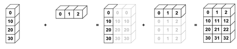
nums_col = np.array([0, 10, 20, 30]).reshape(4, 1)
nums_row = np.array([0, 1, 2])

nums_col + nums_row

array([[ 0,  1,  2],
       [10, 11, 12],
       [20, 21, 22],
       [30, 31, 32]])

import xarray as xr

nums_col = xr.DataArray([0, 10, 20, 30], [('col', [0, 10, 20, 30])])
nums_row = xr.DataArray([0, 1, 2], [('row', [0, 1, 2])])

nums_col + nums_row

<xarray.DataArray (col: 4, row: 3)>
array([[ 0,  1,  2],
       [10, 11, 12],
       [20, 21, 22],
       [30, 31, 32]])
Coordinates:
  * col      (col) int64 0 10 20 30
  * row      (row) int64 0 1 2

Algorithm improvements¶

The instructions to solve the problem.
- Free MIT course on ‘Introduction to algorithms’, video lectures.
Many existing libraries are already optimised (computationally and algorithmically).
- Minimal examples of data structures and algorithms in Python.
- e.g. Find multiple strings in a text.
  - Aho-Corasick algorithm, 25x faster than using regex naively.

Compilers ¶

CPython
- Ahead-Of-Time (AOT) compiler.
  - Statically compiled C extensions.
- General purpose interpreter.
  - Can work on a variety of problems.
- Dynamically typed.
  - Types can change e.g. x = 5, then later x = 'gary'.
PyPy
- Just−In−Time (JIT) compiler (written in Python).
  - Enables optimisations at run time, especially for numerical tasks with repitition and loops.
  - Replaces CPython.
  - Faster, though overheads for start-up and memory.
Numba
- Uses JIT compiler on functions.
  - Converts to fast machine code (LLVM).
  - Uses decorators around functions.
  - Use with the default CPython.
  - Examples for NumPy and Pandas.

from numba import njit

nums = np.arange(1_000_000)

def super_function(nums):
    trace = 0.0
    for num in nums: # loop
        trace += np.cos(num) # numpy
    return nums + trace # broadcasting

%timeit super_function(nums)

1.68 s ± 8.53 ms per loop (mean ± std. dev. of 7 runs, 1 loop each)

@njit # numba decorator
def super_function(nums):
    trace = 0.0
    for num in nums: # loop
        trace += np.cos(num) # numpy
    return nums + trace # broadcasting

%timeit super_function(nums)

15 ms ± 46 µs per loop (mean ± std. dev. of 7 runs, 100 loops each)

Cython
- Compiles to statically typed C/C++.
- Use for any amount of code.
- Use with the default CPython.
- Examples not using IPython, NumPy, Pandas (example below).

import pandas as pd

df = pd.DataFrame({
    "a": np.random.randn(1000),
    "b": np.random.randn(1000),
    "N": np.random.randint(100, 1000, (1000)),
    "x": "x",
})
df.head()

	a	b	N	x
0	-1.860311	-0.551809	288	x
1	0.782267	1.564407	653	x
2	-1.243118	-0.414263	472	x
3	0.107798	-1.261014	312	x
4	-0.524740	0.479698	958	x

def f(x):
    return x * (x - 1)
   

def integrate_f(a, b, N):
    s = 0
    dx = (b - a) / N
    for i in range(N):
        s += f(a + i * dx)
        
    return s * dx

%timeit df.apply(lambda x: integrate_f(x["a"], x["b"], x["N"]), axis=1)

73 ms ± 794 µs per loop (mean ± std. dev. of 7 runs, 10 loops each)

%load_ext Cython

%%cython # only change
def f(x):
    return x * (x - 1)
   

def integrate_f(a, b, N):
    s = 0
    dx = (b - a) / N
    for i in range(N):
        s += f(a + i * dx)
        
    return s * dx

%timeit df.apply(lambda x: integrate_f(x["a"], x["b"], x["N"]), axis=1)

51.7 ms ± 729 µs per loop (mean ± std. dev. of 7 runs, 10 loops each)

%%cython
cdef double f(double x) except? -2:                  # adding types
    return x * (x - 1)
   

cpdef double integrate_f(double a, double b, int N): # adding types
    cdef int i                                       # adding types
    cdef double s, dx                                # adding types
    s = 0
    dx = (b - a) / N
    for i in range(N):
        s += f(a + i * dx)
        
    return s * dx

%timeit df.apply(lambda x: integrate_f(x["a"], x["b"], x["N"]), axis=1)

8.96 ms ± 106 µs per loop (mean ± std. dev. of 7 runs, 100 loops each)

Parallelisation¶

Parallelisation divides a large problem into many smaller ones and solves them simultaneously.
- Divides up the time/space complexity across workers.
- Tasks centrally managed by a scheduler.
- Multi-processing (cores) - useful for compute-bound problems.
- Multi-threading (parts of processes), useful for memory-bound problems.
If need to share memory across chunks:
- Use shared memory (commonly OpenMP, Open Multi-Processing).
- -pe smp np on ARC4
Otherwise:
- Use message passing interface, MPI (commonly OpenMPI).
- -pe ib np on ARC4

Single machine ¶

See the excellent video from Dask creator, Matthew Rocklin, below.

Dask
- Great features.
- Helpful documentation.
- Familiar API.
- Under the hood for many libraries e.g. xarray, iris, scikit-learn.

from dask.distributed import Client
client = Client()
client

ds = xr.open_dataset(
    '/nfs/a68/shared/earlacoa/wrfout_2015_PM_2_DRY_0.25deg.nc',
    chunks={'time': 'auto'} # dask chunks
)

ds.nbytes * (2 ** -30)

%time ds_mean = ds.mean()

%time ds_mean.compute()

ds.close()
client.close()

Multi-threading¶

See the excellent video from Dask creator, Matthew Rocklin, below.

e.g. dask.array (NumPy).

from dask.distributed import Client
client = Client(
    processes=False,
    threads_per_worker=4,
    n_workers=1
)
client

import dask.array as da

my_array = da.random.random(
    (50_000, 50_000),
    chunks=(5_000, 5_000) # dask chunks
)
result = my_array + my_array.T
result

result.compute()

client.close()

Multi-processing¶

See the excellent video from Dask creator, Matthew Rocklin, below.

e.g. dask.dataframe (Pandas).

from dask.distributed import Client
client = Client()
client

import dask
import dask.dataframe as dd

df = dask.datasets.timeseries()
df

type(df)

result = df.groupby('name').x.std()
result

result.visualize()

result_computed = result.compute()

type(result_computed)

client.close()

Interactive on HPC ¶

See the excellent video from Dask creator, Matthew Rocklin, below.

Create or edit the ~/.config/dask/jobqueue.yaml file with that in this directory.
Also, can check the ~/.config/dask/distributed.yaml file with that in this directory.

e.g. dask.bag
- Iterate over a bag of independent objects (embarrassingly parallel).

# in a terminal

# log onto arc4
ssh ${USER}@arc4.leeds.ac.uk

# start an interactive session on a compute node on arc4
qlogin -l h_rt=04:00:00 -l h_vmem=12G

# activate your python environment
conda activate my_python_environment

# echo back the ssh command to connect to this compute node
echo "ssh -N -L 2222:`hostname`:2222 -L 2727:`hostname`:2727 ${USER}@arc4.leeds.ac.uk"

# launch a jupyter lab session on this compute node
jupyter lab --no-browser --ip=`hostname` --port=2222

# in a local terminal
# ssh into the compute node
ssh -N -L 2222:`hostname`:2222 -L 2727:`hostname`:2727 ${USER}@arc4.leeds.ac.uk

# open up a local browser (e.g. chrome)
# go to the jupyter lab session by pasting into the url bar
localhost:2222
    
# can also load the dask dashboard in the browser at localhost:2727

# now the jupyter code
from dask_jobqueue import SGECluster
from dask.distributed import Client

cluster = Client(
    walltime='01:00:00',
    memory='4 G',
    resource_spec='h_vmem=4G',
    scheduler_options={
        'dashboard_address': ':2727',
    },
)

client = Client(cluster)

cluster.scale(jobs=20)
#cluster.adapt(minimum=0, maximum=20)

client

import numpy as np
import dask.bag as db

nums = np.random.randint(low=0, high=100, size=(5_000_000))
nums

def weird_function(nums):
    return chr(nums)

bag = db.from_sequence(nums)
bag = bag.map(weird_function)
bag.visualize()

result = bag.compute()

client.close()
cluster.close()

HPC ¶

Non-interactive.
Create/edit the dask_on_hpc.py file.
Submit to the queue using qsub dask_on_hpc.bash.

Profile parallel code¶

Example visualisation of profiler.

Suitable data types for parallel computing¶

Parquet creates efficient tabular data (e.g. dataframes), useful for parallel computing.
- Accessed via pyarrow.
Zarr creates compressed, chunked, N-dimensional arrays, designed for use in parallel computing.

GPUs¶

GPUs (Graphics Processing Units) are optimised for numerical operations, while CPUs perform general computation.
cuPy (NumPy).

import cupy as cp
x = cp.arange(6).reshape(2, 3).astype('f')
x.sum(axis=1)

cuDF (Pandas).
Can run in parallel.
- GPUs available on ARC4.

Recommendations¶

Check code is correct and optimisation is needed.
Profile to find bottlenecks.
- Jupyter Lab: %%timeit and %%memit.
- Line-by-line: line_profiler and memory_profiler.
Optimise code and data.
- Data structures.
- Use existing optimised libraries (algorithms).
- Vectorisation (instead of loops).
- Lazy loading and execution.
- If numerically intensive problem:
  - All code, use PyPy/GPUs.
  - Specific functions, use Numba.
- If need static typing, use Cython.
Parallelise.
- Use multi-processing (don’t need to worry about GIL).
- Use Dask (Coiled).

Further information¶

Helpful resources

Why is Python slow?, Anthony Shaw, PyCon 2020. CPython Internals.
Luciano Ramalho, Fluent Python, Clear, Concise, and Effective Programming, 2015. O’Reilly Media, Inc.
Jake VanderPlas, Python Data Science Handbook, 2016. O’Reilly Media, Inc.
Pangeo, talk - Python libraries that work well together and build on each other, especially for big data geosciences (e.g. NumPy, Pandas, xarray, Dask, Numba, Jupyter).
Concurrency can also run different tasks together, but work is not done at the same time.
Asynchronous (multi-threading), useful for massive scaling, threads controlled explicitly.
MIT course on ‘Introduction to algorithms’, video lectures.
PythonSpeed.com, Itamar Turner-Trauring
Writing faster Python, Sebastian Witowski, Euro Python 2016
AlgoExpert

Other things that may help save time in the long run:

Tips to speed up Python¶

Contents¶

Hang on, don’t optimise too early¶

How fast is it?¶

How fast could it go?¶

Potential improvements¶

Append to lists, rather than concatenating¶

Move loop-invariants outside loops¶

Use built-in functions¶

Use optimal data types¶

Reduce repeated calculations with caching¶

Use vectorisation instead of loops¶

Algorithm improvements¶

Compilers¶

Lazy loading and execution¶

Parallelisation¶

Single machine¶

Multi-threading¶

Multi-processing¶

Interactive on HPC¶

HPC¶

Profile parallel code¶

Suitable data types for parallel computing¶

GPUs¶

Recommendations¶

Further information¶

Use built-in functions ¶

Use optimal data types ¶

Reduce repeated calculations with caching ¶

Compilers ¶

Lazy loading and execution ¶

Single machine ¶

Interactive on HPC ¶

HPC ¶