Distributed¶

Note

If you’re in COLAB or have a local CUDA GPU, you can follow along with the more computationally intensive training in this lesson.

For those in COLAB, ensure the session is using a GPU by going to: Runtime > Change runtime type > Hardware accelerator = GPU.

# if you're using colab, then install the required modules
import sys

IN_COLAB = "google.colab" in sys.modules
if IN_COLAB:
    %pip install --quiet --upgrade ray

Distributing training over multiple devices generally uses either:

Data parallelism
- Split the data over multiple devices.
- Single model copied to multiple devices.
- Useful for big data.
- Simpler.
Model parallelism
- Split the model over multiple devices.
- Single data copied to multiple devices.
- Can be useful for big models (for some architectures).
- More complex.

This lesson focuses on data parallelism.

Ray Train ¶

Ray Train is a useful tool for distributed deep learning training for TensorFlow (Keras) and PyTorch.

It handles the set up for you (e.g., TF_CONFIG in TensorFlow).

There are a range of examples here.

Warning

Note, Ray doesn’t currently work on POWER9 machines e.g., Bede. See, GitHub issue.

Example: TensorFlow (Keras) MNIST ¶

import argparse
import json
import os

import numpy as np
import ray
import tensorflow as tf
from ray.train import Trainer
from tensorflow.keras.callbacks import Callback

2022-04-25 10:35:22.628359: W tensorflow/stream_executor/platform/default/dso_loader.cc:64] Could not load dynamic library 'libcudart.so.11.0'; dlerror: libcudart.so.11.0: cannot open shared object file: No such file or directory
2022-04-25 10:35:22.628392: I tensorflow/stream_executor/cuda/cudart_stub.cc:29] Ignore above cudart dlerror if you do not have a GPU set up on your machine.

Define callback for reporting ¶

class TrainReportCallback(Callback):
    def on_epoch_end(self, epoch, logs=None):
        ray.train.report(**logs)

Set up the dataset and model¶

The dataset will be split (sharded) across the workers.

Tip

The default auto-sharding by FILE can cause warning messages if the data is in one file. Instead, you can specify to auto-shard by data using: tf.data.experimental.AutoShardPolicy.DATA (which it will fall back to anyway).

def mnist_dataset(batch_size):
    (x_train, y_train), _ = tf.keras.datasets.mnist.load_data()
    # The `x` arrays are in uint8 and have values in the [0, 255] range.
    # You need to convert them to float32 with values in the [0, 1] range.
    x_train = x_train / np.float32(255)
    y_train = y_train.astype(np.int64)
    ds_train = (
        tf.data.Dataset.from_tensor_slices((x_train, y_train))
        .shuffle(60000)
        .repeat()
        .batch(batch_size)
    )

    options = tf.data.Options()
    options.experimental_distribute.auto_shard_policy = (
        tf.data.experimental.AutoShardPolicy.DATA
    )
    ds_train = ds_train.with_options(options)

    return ds_train

When building the model, a config keyword argument is added to get different options such as the learning rate.

def build_and_compile_cnn_model(config):
    learning_rate = config.get("lr", 0.001)
    model = tf.keras.Sequential(
        [
            tf.keras.Input(shape=(28, 28)),
            tf.keras.layers.Reshape(target_shape=(28, 28, 1)),
            tf.keras.layers.Conv2D(32, 3, activation="relu"),
            tf.keras.layers.Flatten(),
            tf.keras.layers.Dense(128, activation="relu"),
            tf.keras.layers.Dense(10),
        ]
    )
    model.compile(
        loss=tf.keras.losses.SparseCategoricalCrossentropy(from_logits=True),
        optimizer=tf.keras.optimizers.SGD(learning_rate=learning_rate),
        metrics=["accuracy"],
    )
    return model

Set up the training function for a single worker¶

This also uses the config argument.

def train_func(config):
    batch_size = 64
    single_worker_dataset = mnist_dataset(batch_size)
    single_worker_model = build_and_compile_cnn_model(config)
    single_worker_model.fit(
        single_worker_dataset,
        epochs=config["epochs"],
        steps_per_epoch=70,
        verbose=False,
    )

Now, you configure training using the config parameter.

config = {"epochs": 3}

train_func(config)

2022-04-25 10:35:24.607304: W tensorflow/stream_executor/platform/default/dso_loader.cc:64] Could not load dynamic library 'libcuda.so.1'; dlerror: libcuda.so.1: cannot open shared object file: No such file or directory
2022-04-25 10:35:24.607350: W tensorflow/stream_executor/cuda/cuda_driver.cc:269] failed call to cuInit: UNKNOWN ERROR (303)
2022-04-25 10:35:24.607375: I tensorflow/stream_executor/cuda/cuda_diagnostics.cc:156] kernel driver does not appear to be running on this host (fv-az39-99): /proc/driver/nvidia/version does not exist
2022-04-25 10:35:24.607739: I tensorflow/core/platform/cpu_feature_guard.cc:151] This TensorFlow binary is optimized with oneAPI Deep Neural Network Library (oneDNN) to use the following CPU instructions in performance-critical operations:  AVX2 AVX512F FMA
To enable them in other operations, rebuild TensorFlow with the appropriate compiler flags.
2022-04-25 10:35:24.608834: W tensorflow/core/framework/cpu_allocator_impl.cc:82] Allocation of 188160000 exceeds 10% of free system memory.
2022-04-25 10:35:24.770969: W tensorflow/core/framework/cpu_allocator_impl.cc:82] Allocation of 188160000 exceeds 10% of free system memory.

Set the distributed strategy ¶

**Set the global batch size**¶

Each worker will process the same size batch as in the single-worker code.

Hence, the global batch size will be the single-worker batch size multiplied by the number of workers.

Choose your TensorFlow distributed training strategy¶

The MirroredStrategy copies all of the model’s variables (parameters) to each device on one machine.

This ensures all replicas across the workers are identical.

Then it combines the gradients from all devices and applies the combined value to all copies of the model.

The MultiWorkerMirroredStrategy is similar to the MirroredStrategy, apart from that it can work for devices on multiple machines.

In this example, we’ll use the MultiWorkerMirroredStrategy.

Within the strategy scope context manager, you build and compile the model.

def train_func(config):
    per_worker_batch_size = config.get("batch_size", 64)
    epochs = config.get("epochs", 3)
    steps_per_epoch = config.get("steps_per_epoch", 70)

    tf_config = json.loads(os.environ["TF_CONFIG"])
    num_workers = len(tf_config["cluster"]["worker"])

    strategy = tf.distribute.MultiWorkerMirroredStrategy()

    global_batch_size = per_worker_batch_size * num_workers
    multi_worker_dataset = mnist_dataset(global_batch_size)

    with strategy.scope():
        # model building/compiling need to be within strategy.scope()
        multi_worker_model = build_and_compile_cnn_model(config)

    history = multi_worker_model.fit(
        multi_worker_dataset,
        epochs=epochs,
        steps_per_epoch=steps_per_epoch,
        callbacks=[TrainReportCallback()],
        verbose=False,
    )
    results = history.history
    return results

Create Ray Train Trainer ¶

The Trainer manages state and training.

Ray Train enables different backend options e.g., tensorflow.

def train_tensorflow_mnist(num_workers=1, use_gpu=False, epochs=4):
    trainer = Trainer(backend="tensorflow", num_workers=num_workers, use_gpu=use_gpu)
    trainer.start()
    results = trainer.run(
        train_func=train_func, config={"lr": 1e-3, "batch_size": 64, "epochs": epochs}
    )
    trainer.shutdown()
    print(f"Results: {results[0]}")

Run the training ¶

Initialise and shutdown the Ray client:

# ray.init()

# cpu
# train_tensorflow_mnist()

# gpu
# train_tensorflow_mnist(use_gpu=True)

# ray.shutdown()

Submit the job to HPC¶

This Python script is in full here.

CPUs¶

An example job submission script is (also here):

#!/bin/bash
#$ -cwd -V
#$ -l h_rt=00:30:00
#$ -pe smp 12
#$ -l h_vmem=6G

# activate conda and add to library path
conda activate intro_ml
export LD_LIBRARY_PATH=$LD_LIBRARY_PATH:$CONDA_PREFIX/lib

# run the CPU script
python tensorflow_ray_train_mnist_example.py --num-workers 12 --epochs 100

Warning

Sometimes the LD_LIBRARY_PATH variable will not include the path to the conda environment, resulting it in being unable to find some libraries e.g., TensorFlow, cuDNN.

To resolve this, in your script append the path to your activated conda environment to the LD_LIBRARY_PATH variable using:

export LD_LIBRARY_PATH=$LD_LIBRARY_PATH:$CONDA_PREFIX/lib

Note

These scripts are based on a personal miniconda with the environment activated at the terminal and the terminal LD_LIBRARY_PATH updated.

There are other options e.g., using the Anaconda distribution installed on ARC.

To change the number of workers (either CPUs or GPUs), set the --num-workers argument.

Ensure that the scheduler request matches this number e.g.,:

For 12 CPU workers, use --num-workers 12 and #$ -pe smp 12.
For 2 GPU workers, use --num-workers 2 and #$ -l coproc_v100=2.
- To use GPUs, you will also need the --use-gpu True flag.

In this simple example using 12 CPUs, the job efficiency was (using qacct -j <JOBID>):

Efficiency = 100 * cpu / (ru_wallclock * slots)
Efficiency = 100 * 10214 / (928 * 12)
Efficiency = 92 %

92% is good.

GPU(s)¶

Note

The tests below were for a NVIDIA V100 with 32 GB of memory.

An example job submission script is (also here):

#!/bin/bash
#$ -cwd -V
#$ -l h_rt=00:15:00
#$ -l coproc_v100=1

# activate conda and add to library path
conda activate swd8_intro_ml 
export LD_LIBRARY_PATH=$LD_LIBRARY_PATH:$CONDA_PREFIX/lib

# start the efficiency log for the GPU
nvidia-smi dmon -d 10 -s um -i 0 > efficiency_log &

# run the GPU script
python tensorflow_ray_train_mnist_example.py --use-gpu True --num-workers 1 --epochs 100

# stop the efficiency log
kill %1

You can check the efficiency of your GPU job using the NVIDIA System Management Interface i.e., nvidia-smi.

dmon is for device monitoring.
-d X records the metrics every X seconds.
-s um is the metrics to sample, where u = utilisation and m = memory.
-i 0 is the device number, where 0 = first gpu. For multiple devices, add them separated by commas e.g., -i 0,1.

Then you can view the results from the efficiency_log:

# gpu    sm   mem   enc   dec    fb  bar1
# Idx     %     %     %     %    MB    MB
    0     0     0     0     0     0     2
    0     0     0     0     0     0     2
    0     0     0     0     0 31880     5
    0    34    15     0     0 31932     5

The main columns are sm (for utilisation %) and mem (for memory %).

Here, the job utilised approximately 35% of the GPU and 15% of its memory. (The first few rows are blank as the GPU was idle while the CPU downloaded the data.)

That’s quite low, though this was for a simple MNIST example.

A more complex problem will likely utilise the GPU better.

Example: TensorFlow (Keras) transfer learning ¶

In lesson 4, we looked at a TensorFlow (Keras) transfer learning example. To use this script with Ray Train, you primarily need to create the dataset pipeline and model creation functions. You can use the examples here as a foundation. The full script for this example is here.

Running this code on a single GPU utilised approximately 90% of the GPU and 45% of its memory.

This is good.

Multiple GPUs is not needed for this transfer learning example.

However, if we set the pre-trained model to trainable (rather than being frozen), then this may be suitable for using multiple workers.

To do this, we set trainable=True within the assignment of feature_extractor_layer like this:

feature_extractor_layer = hub.KerasLayer(
    feature_extractor_model,
    input_shape=(IMAGE_HEIGHT, IMAGE_WIDTH, 3),
    trainable=True,  # this line is the only change
)

Then we change the submission script to:

Request 2 workers in the Ray Train flag for the Python script call using --num-workers 2.
Request 2 GPUs from the scheduler using #$ -l coproc_v100=2.
Monitor both GPUs using nvidia-smi dmon -i 0,1.

This then utilised both devices well, with both using approximately 90% of the GPU’s compute and 50% of their memory.

Tip

To utilise GPU(s) efficiently, try to match the resources requested to what your problem requires e.g., the model of GPU, the memory it has, etc.

PyTorch (Lightning)¶

PyTorch Lightning comes with great built-in functionality to scale to multiple GPUs.

First though, we should check that the problem requires these resources.

A simple example for MNIST utilises about 8% of a single V100 GPU.

The PyTorch Lightning transfer learning example (lesson 4) utilises about 15% of a single V100 GPU (full script here).

To demonstrate running this transfer learning example over multiple GPUs, we could unfreeze the pre-trained model to increase the workload.

This is normally not recommended, though is useful for demonstration purposes here of a complex model.

To unfreeze the pre-trained model:

Set trainer.finetune(strategy="unfreeze").
This is also the default setting.

Then the steps to run over multiple GPUs are:

Specify the data parallel strategy in the Trainer:

from pytorch_lightning.strategies import DDPStrategy

trainer = flash.Trainer(
    max_epochs=100,
    accelerator="gpu",
    devices=torch.cuda.device_count(),
    strategy=DDPStrategy(find_unused_parameters=False),
)

Note, setting find_unused_parameters=False can improve performance.

Set the scheduler to use multiple GPUs:
- e.g., #$ -l coproc_v100=2.
Adding GPU monitoring for multiple GPUs:
- e.g., nvidia-smi dmon -i 0,1.

This utilised 2 V100 GPUs at approximately 40%. This isn’t great, though it demonstrates the ease of distributed training with PyTorch Lightning.

Jupyter Notebook to HPC¶

Once you’ve finished testing out different ideas locally in a Jupyter Notebook, you can then convert this to an executable script to run on a HPC.

This is because the HPCs (currently accessible at Leeds, at least) are suitable for non-interactive batch jobs.

The steps are to:

Clean non-essential code
Refactor Jupyter Notebook code into functions
Create a Python script
Create submission script
(Optional) Create unit tests

Clean non-essential code¶

Some code added during the experimentation phase was only needed to test out ideas and explore the data.

This non-essential code can be removed to make it more maintainable and performant.

Let’s use the example from the TensorFlow Datasets MNIST example we saw in Lesson 3.

import os

import matplotlib.pyplot as plt
import tensorflow as tf
import tensorflow_datasets as tfds

# global setup
tf.keras.utils.set_random_seed(42)
print("Num GPUs Available: ", len(tf.config.list_physical_devices("GPU")))
AUTOTUNE = tf.data.AUTOTUNE
NUM_EPOCHS = 5

# download the data
(ds_train, ds_val, ds_test), ds_info = tfds.load(
    "mnist",
    split=["train[:80%]", "train[80%:90%]", "train[90%:]"],
    shuffle_files=True,
    as_supervised=True,
    with_info=True,
)

print(ds_train)
print(ds_info)

# preprocess the data
def normalise_image(image, label):
    return tf.cast(image, tf.float32) / 255.0, label


# create data pipelines
def training_pipeline(ds_train):
    ds_train = ds_train.map(normalise_image, num_parallel_calls=AUTOTUNE)
    ds_train = ds_train.cache()
    ds_train = ds_train.shuffle(ds_info.splits["train"].num_examples)
    ds_train = ds_train.batch(128)
    ds_train = ds_train.prefetch(AUTOTUNE)
    return ds_train


def test_pipeline(ds_test):
    ds_test = ds_test.map(normalise_image, num_parallel_calls=AUTOTUNE)
    ds_test = ds_test.batch(128)
    ds_test = ds_test.cache()
    ds_test = ds_test.prefetch(AUTOTUNE)
    return ds_test


ds_train = training_pipeline(ds_train)
ds_val = training_pipeline(ds_val)
ds_test = test_pipeline(ds_test)


# create the model
inputs = tf.keras.Input(shape=(28, 28, 1), name="inputs")
x = tf.keras.layers.Flatten(name="flatten")(inputs)
x = tf.keras.layers.Dense(128, activation="relu", name="layer1")(x)
x = tf.keras.layers.Dropout(0.2)(x)
x = tf.keras.layers.Dense(128, activation="relu", name="layer2")(x)
outputs = tf.keras.layers.Dense(10, name="outputs")(x)

model = tf.keras.Model(inputs, outputs, name="functional")

# view the model
model.summary()

# compile the model
model.compile(
    optimizer=tf.keras.optimizers.Adam(),
    loss=tf.keras.losses.SparseCategoricalCrossentropy(from_logits=True),
    metrics=[tf.keras.metrics.SparseCategoricalAccuracy(name="accuracy")],
)

# train the model
history = model.fit(
    ds_train,
    validation_data=ds_val,
    epochs=NUM_EPOCHS,
    verbose=False,
)

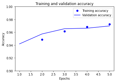
# plot the model accuracy
epochs_range = range(1, NUM_EPOCHS + 1)

plt.plot(epochs_range, history.history["accuracy"], "bo", label="Training accuracy")
plt.plot(
    epochs_range, history.history["val_accuracy"], "b", label="Validation accuracy"
)
plt.title("Training and validation accuracy")
plt.xlabel("Epochs")
plt.ylabel("Accuracy")
plt.ylim([0.9, 1.0])
plt.legend()
plt.show()

# save the model
path_models = f"{os.getcwd()}/models"
model.save(f"{path_models}/model_tf_mnist")

Num GPUs Available:  0
<_OptionsDataset element_spec=(TensorSpec(shape=(28, 28, 1), dtype=tf.uint8, name=None), TensorSpec(shape=(), dtype=tf.int64, name=None))>
tfds.core.DatasetInfo(
    name='mnist',
    full_name='mnist/3.0.1',
    description="""
    The MNIST database of handwritten digits.
    """,
    homepage='http://yann.lecun.com/exdb/mnist/',
    data_path='/home/runner/tensorflow_datasets/mnist/3.0.1',
    download_size=11.06 MiB,
    dataset_size=21.00 MiB,
    features=FeaturesDict({
        'image': Image(shape=(28, 28, 1), dtype=tf.uint8),
        'label': ClassLabel(shape=(), dtype=tf.int64, num_classes=10),
    }),
    supervised_keys=('image', 'label'),
    disable_shuffling=False,
    splits={
        'test': <SplitInfo num_examples=10000, num_shards=1>,
        'train': <SplitInfo num_examples=60000, num_shards=1>,
    },
    citation="""@article{lecun2010mnist,
      title={MNIST handwritten digit database},
      author={LeCun, Yann and Cortes, Corinna and Burges, CJ},
      journal={ATT Labs [Online]. Available: http://yann.lecun.com/exdb/mnist},
      volume={2},
      year={2010}
    }""",
)

Model: "functional"

_________________________________________________________________

 Layer (type)                Output Shape              Param #

=================================================================

 inputs (InputLayer)         [(None, 28, 28, 1)]       0

 flatten (Flatten)           (None, 784)               0

 layer1 (Dense)              (None, 128)               100480

 dropout (Dropout)           (None, 128)               0

 layer2 (Dense)              (None, 128)               16512

 outputs (Dense)             (None, 10)                1290

=================================================================

Total params: 118,282

Trainable params: 118,282

Non-trainable params: 0

_________________________________________________________________

2022-04-25 10:35:40.356423: W tensorflow/python/util/util.cc:368] Sets are not currently considered sequences, but this may change in the future, so consider avoiding using them.

INFO:tensorflow:Assets written to: /home/runner/work/intro_ml/intro_ml/docs/models/model_tf_mnist/assets

INFO:tensorflow:Assets written to: /home/runner/work/intro_ml/intro_ml/docs/models/model_tf_mnist/assets

We can now remove the non-essential code, as the experimentation phase is complete.

Here, this included:

Removing data information from the download.
Removing unrequired print statements.
Viewing model summary.
Removing/replacing plots with text output.

import os

import matplotlib.pyplot as plt
import tensorflow as tf
import tensorflow_datasets as tfds

# global setup
tf.keras.utils.set_random_seed(42)
print("Num GPUs Available: ", len(tf.config.list_physical_devices("GPU")))
AUTOTUNE = tf.data.AUTOTUNE
NUM_EPOCHS = 5

# download the data
(ds_train, ds_val, ds_test) = tfds.load(
    "mnist",
    split=["train[:80%]", "train[80%:90%]", "train[90%:]"],
    shuffle_files=True,
    as_supervised=True,
    with_info=False,
)

# preprocess the data
def normalise_image(image, label):
    return tf.cast(image, tf.float32) / 255.0, label


# create data pipelines
def training_pipeline(ds_train):
    ds_train = ds_train.map(normalise_image, num_parallel_calls=AUTOTUNE)
    ds_train = ds_train.cache()
    ds_train = ds_train.shuffle(ds_info.splits["train"].num_examples)
    ds_train = ds_train.batch(128)
    ds_train = ds_train.prefetch(AUTOTUNE)
    return ds_train


def test_pipeline(ds_test):
    ds_test = ds_test.map(normalise_image, num_parallel_calls=AUTOTUNE)
    ds_test = ds_test.batch(128)
    ds_test = ds_test.cache()
    ds_test = ds_test.prefetch(AUTOTUNE)
    return ds_test


ds_train = training_pipeline(ds_train)
ds_val = training_pipeline(ds_val)
ds_test = test_pipeline(ds_test)


# create the model
inputs = tf.keras.Input(shape=(28, 28, 1), name="inputs")
x = tf.keras.layers.Flatten(name="flatten")(inputs)
x = tf.keras.layers.Dense(128, activation="relu", name="layer1")(x)
x = tf.keras.layers.Dropout(0.2)(x)
x = tf.keras.layers.Dense(128, activation="relu", name="layer2")(x)
outputs = tf.keras.layers.Dense(10, name="outputs")(x)

model = tf.keras.Model(inputs, outputs, name="functional")

# compile the model
model.compile(
    optimizer=tf.keras.optimizers.Adam(),
    loss=tf.keras.losses.SparseCategoricalCrossentropy(from_logits=True),
    metrics=[tf.keras.metrics.SparseCategoricalAccuracy(name="accuracy")],
)

# train the model
history = model.fit(
    ds_train,
    validation_data=ds_val,
    epochs=NUM_EPOCHS,
    verbose=False,
)

# view the model accuracy
print(f"Training accuracy: {[round(num, 2) for num in history.history['accuracy']]}")
print(
    f"Validation accuracy: {[round(num, 2) for num in history.history['val_accuracy']]}"
)

# save the model
path_models = f"{os.getcwd()}/models"
model.save(f"{path_models}/model_tf_mnist")

Num GPUs Available:  0

Training accuracy: [0.88, 0.95, 0.96, 0.97, 0.97]
Validation accuracy: [0.94, 0.96, 0.97, 0.97, 0.97]

INFO:tensorflow:Assets written to: /home/runner/work/intro_ml/intro_ml/docs/models/model_tf_mnist/assets

INFO:tensorflow:Assets written to: /home/runner/work/intro_ml/intro_ml/docs/models/model_tf_mnist/assets

Refactor Jupyter Notebook code into functions¶

Now, any code that is not already in functions, can be refactored into functions.

Modularising the code like this helps with diagnosing errors and creating tests.

Here, we added functions for:

Downloading the data.
Creating and compiling the model.
Training the model.
Saving the model.
A main function for the whole workflow.

import os

import matplotlib.pyplot as plt
import tensorflow as tf
import tensorflow_datasets as tfds

# global setup
tf.keras.utils.set_random_seed(42)
print("Num GPUs Available: ", len(tf.config.list_physical_devices("GPU")))
AUTOTUNE = tf.data.AUTOTUNE
NUM_EPOCHS = 5

# download the data
def download_data():
    (ds_train, ds_val, ds_test) = tfds.load(
        "mnist",
        split=["train[:80%]", "train[80%:90%]", "train[90%:]"],
        shuffle_files=True,
        as_supervised=True,
        with_info=False,
    )
    return ds_train, ds_val, ds_test


# preprocess the data
def normalise_image(image, label):
    return tf.cast(image, tf.float32) / 255.0, label


# create data pipelines
def training_pipeline(ds_train):
    ds_train = ds_train.map(normalise_image, num_parallel_calls=AUTOTUNE)
    ds_train = ds_train.cache()
    ds_train = ds_train.shuffle(ds_info.splits["train"].num_examples)
    ds_train = ds_train.batch(128)
    ds_train = ds_train.prefetch(AUTOTUNE)
    return ds_train


def test_pipeline(ds_test):
    ds_test = ds_test.map(normalise_image, num_parallel_calls=AUTOTUNE)
    ds_test = ds_test.batch(128)
    ds_test = ds_test.cache()
    ds_test = ds_test.prefetch(AUTOTUNE)
    return ds_test


# create and compile the model
def create_and_compile_model():
    inputs = tf.keras.Input(shape=(28, 28, 1), name="inputs")
    x = tf.keras.layers.Flatten(name="flatten")(inputs)
    x = tf.keras.layers.Dense(128, activation="relu", name="layer1")(x)
    x = tf.keras.layers.Dropout(0.2)(x)
    x = tf.keras.layers.Dense(128, activation="relu", name="layer2")(x)
    outputs = tf.keras.layers.Dense(10, name="outputs")(x)

    model = tf.keras.Model(inputs, outputs, name="functional")

    model.compile(
        optimizer=tf.keras.optimizers.Adam(),
        loss=tf.keras.losses.SparseCategoricalCrossentropy(from_logits=True),
        metrics=[tf.keras.metrics.SparseCategoricalAccuracy(name="accuracy")],
    )

    return model


# train the model
def train_model():
    history = model.fit(
        ds_train,
        validation_data=ds_val,
        epochs=NUM_EPOCHS,
        verbose=False,
    )
    return history


# save the model
def save_model(model):
    path_models = f"{os.getcwd()}/models"
    model.save(f"{path_models}/model_tf_mnist")


# combine the functions in a call to main
def main():
    ds_train, ds_val, ds_test = download_data()

    ds_train = training_pipeline(ds_train)
    ds_val = training_pipeline(ds_val)
    ds_test = test_pipeline(ds_test)

    model = create_and_compile_model()
    history = train_model()
    save_model(model)


# run the functions
main()

# view the model accuracy
print(f"Training accuracy: {[round(num, 2) for num in history.history['accuracy']]}")
print(
    f"Validation accuracy: {[round(num, 2) for num in history.history['val_accuracy']]}"
)

Num GPUs Available:  0

INFO:tensorflow:Assets written to: /home/runner/work/intro_ml/intro_ml/docs/models/model_tf_mnist/assets

INFO:tensorflow:Assets written to: /home/runner/work/intro_ml/intro_ml/docs/models/model_tf_mnist/assets

Training accuracy: [0.88, 0.95, 0.96, 0.97, 0.97]
Validation accuracy: [0.94, 0.96, 0.97, 0.97, 0.97]

Create a Python script¶

First, the call to main() should be placed inside a conditional invocation i.e.,:

if __name__ == '__main__':
    main()

Now, the script can be called from a terminal by running python script.py.

Then, the rest of the code can be converted by either:

Option 1 (recommended)¶

Convert a single cell to a script using the %%writefile IPython magic command.

%%writefile jupyter-to-hpc_tf-mnist-example.py

import os

import matplotlib.pyplot as plt
import tensorflow as tf
import tensorflow_datasets as tfds

# global setup
tf.keras.utils.set_random_seed(42)
print("Num GPUs Available: ", len(tf.config.list_physical_devices("GPU")))
AUTOTUNE = tf.data.AUTOTUNE
NUM_EPOCHS = 5

# download the data
def download_data():
    (ds_train, ds_val, ds_test) = tfds.load(
        "mnist",
        split=["train[:80%]", "train[80%:90%]", "train[90%:]"],
        shuffle_files=True,
        as_supervised=True,
        with_info=False,
    )
    return ds_train, ds_val, ds_test


# preprocess the data
def normalise_image(image, label):
    return tf.cast(image, tf.float32) / 255.0, label


# create data pipelines
def training_pipeline(ds_train):
    ds_train = ds_train.map(normalise_image, num_parallel_calls=AUTOTUNE)
    ds_train = ds_train.cache()
    ds_train = ds_train.shuffle(ds_info.splits["train"].num_examples)
    ds_train = ds_train.batch(128)
    ds_train = ds_train.prefetch(AUTOTUNE)
    return ds_train


def test_pipeline(ds_test):
    ds_test = ds_test.map(normalise_image, num_parallel_calls=AUTOTUNE)
    ds_test = ds_test.batch(128)
    ds_test = ds_test.cache()
    ds_test = ds_test.prefetch(AUTOTUNE)
    return ds_test


# create and compile the model
def create_and_compile_model():
    inputs = tf.keras.Input(shape=(28, 28, 1), name="inputs")
    x = tf.keras.layers.Flatten(name="flatten")(inputs)
    x = tf.keras.layers.Dense(128, activation="relu", name="layer1")(x)
    x = tf.keras.layers.Dropout(0.2)(x)
    x = tf.keras.layers.Dense(128, activation="relu", name="layer2")(x)
    outputs = tf.keras.layers.Dense(10, name="outputs")(x)

    model = tf.keras.Model(inputs, outputs, name="functional")

    model.compile(
        optimizer=tf.keras.optimizers.Adam(),
        loss=tf.keras.losses.SparseCategoricalCrossentropy(from_logits=True),
        metrics=[tf.keras.metrics.SparseCategoricalAccuracy(name="accuracy")],
    )

    return model


# train the model
def train_model():
    history = model.fit(
        ds_train,
        validation_data=ds_val,
        epochs=NUM_EPOCHS,
        verbose=False,
    )
    return history


# save the model
def save_model(model):
    path_models = f"{os.getcwd()}/models"
    model.save(f"{path_models}/model_tf_mnist")


# combine the functions in a call to main
def main():
    ds_train, ds_val, ds_test = download_data()

    ds_train = training_pipeline(ds_train)
    ds_val = training_pipeline(ds_val)
    ds_test = test_pipeline(ds_test)

    model = create_and_compile_model()
    history = train_model()
    save_model(model)


if __name__ == "__main__":
    # run the functions
    main()

    # view the model accuracy
    print(
        f"Training accuracy: {[round(num, 2) for num in history.history['accuracy']]}"
    )
    print(
        f"Validation accuracy: {[round(num, 2) for num in history.history['val_accuracy']]}"
    )

Overwriting jupyter-to-hpc_tf-mnist-example.py

Option 2¶

Convert the entire notebook to a script using the nbconvert package:

jupyter nbconvert "my_notebook.ipynb" --to script

Option 3¶

Convert the entire notebook to a script using the Jupyter menu.

From within the Jupyter Notebook, click File > Save and Export Notebook As ... > Executable Script.

This should convert the Jupyter Notebook to a .py file, and download it locally.

Create submission script¶

For your HPC (e.g., ARC4), create the submission script.

For example:

#!/bin/bash
#$ -cwd
#$ -l h_rt=00:05:00
#$ -l coproc_v100=1

conda activate intro_ml 
export LD_LIBRARY_PATH=$LD_LIBRARY_PATH:$CONDA_PREFIX/lib  # (sometimes required)

python jupyter-to-hpc_tf-mnist-example.py

Ensure both of these files are on the HPC, alongside the corresponding conda environment.

(Optional) Create unit tests¶

It’s good practise to write tests for your code.

pytest are NumPy are both good, commonly-used tools for testing in Python.

There are various levels, types, and methods of testing.

For example, you could unit test individual functions, like the downloading and splitting of data:

import numpy as np

def test_split_data(ds_train, ds_val, ds_test):
    num_samples_train = len(ds_train)
    num_samples_val = len(ds_val)
    num_samples_test = len(ds_test)
    
    num_samples = num_samples_train + num_samples_val + num_samples_test
    
    np.testing.assert_almost_equal(num_samples_train / num_samples, 0.8, decimal=3)
    np.testing.assert_almost_equal(num_samples_val / num_samples, 0.1, decimal=3)
    np.testing.assert_almost_equal(num_samples_test / num_samples, 0.1, decimal=3)
    

test_split_data(ds_train, ds_val, ds_test)

You could also perform system testing. For example, checking the final validation accuracy is above a threshold:

def test_final_val_accuracy_above_threshold(threshold):
    assert history.history['val_accuracy'][-1] >= threshold
    
test_final_val_accuracy_above_threshold(0.96)

Questions¶

Question 1

What are the two ways to parallelise machine learning, and which way is simpler?

Question 2

How can you check the efficiency of a CPU job?

Question 3

How can you check the efficiency of a GPU job?

Question 4

What tools can help distribute TensorFlow and PyTorch code?

Question 5

In general, what should the batch size be for distributed work?

Question 6

What are some good steps for moving Jupyter Notebook code to HPC?

Solutions ¶

Further information¶

Good practices¶

Ensure everything works on a single device first, before going distributed.
Ensure that you need the overhead of distributing over multiple GPUs e.g., could you instead use 1 GPU and model checkpointing/transfer learning?
Ensure that the problem is complex enough to utilise multiple GPUs efficiently.
Batch the dataset with the global batch size e.g., for 8 devices each capable of a batch of 64 use the global batch size of 512 (= 8 * 64).
Distributed training on PyTorch Lightning
Performance tips from PyTorch

Other options¶

Horovod
- A library to make distributed deep learning fast and easy to use.
DeepSpeed
- A deep learning optimization library that makes distributed training easy, efficient, and effective.
FairScale
- A PyTorch extension library for high performance and large scale training.

SWD8: Introduction to Machine Learning

Distributed

Contents

Distributed¶

Ray Train ¶

Example: TensorFlow (Keras) MNIST ¶

Define callback for reporting ¶

Set up the dataset and model¶

Set up the training function for a single worker¶

Set the distributed strategy ¶

**Set the global batch size**¶

Choose your TensorFlow distributed training strategy¶

Create Ray Train Trainer ¶

Run the training ¶

Submit the job to HPC¶

CPUs¶

GPU(s)¶

Example: TensorFlow (Keras) transfer learning ¶

PyTorch (Lightning)¶

Jupyter Notebook to HPC¶

Clean non-essential code¶

Refactor Jupyter Notebook code into functions¶

Create a Python script¶

Option 1 (recommended)¶

Option 2¶

Option 3¶

Create submission script¶

(Optional) Create unit tests¶

Questions¶

Solutions ¶

Key Points¶

Further information¶

Good practices¶

Other options¶

Resources¶

SWD8: Introduction to Machine Learning

Distributed

Contents

Distributed¶

Ray Train¶

Example: TensorFlow (Keras) MNIST¶

Define callback for reporting¶

Set up the dataset and model¶

Set up the training function for a single worker¶

Set the distributed strategy¶

Set the global batch size¶

Choose your TensorFlow distributed training strategy¶

Create Ray Train Trainer¶

Run the training¶

Submit the job to HPC¶

CPUs¶

GPU(s)¶

Example: TensorFlow (Keras) transfer learning¶

PyTorch (Lightning)¶

Jupyter Notebook to HPC¶

Clean non-essential code¶

Refactor Jupyter Notebook code into functions¶

Create a Python script¶

Option 1 (recommended)¶

Option 2¶

Option 3¶

Create submission script¶

(Optional) Create unit tests¶

Questions¶

Solutions¶

Key Points¶

Further information¶

Good practices¶

Other options¶

Resources¶

Ray Train ¶

Example: TensorFlow (Keras) MNIST ¶

Define callback for reporting ¶

Set the distributed strategy ¶

**Set the global batch size**¶

Create Ray Train Trainer ¶

Run the training ¶

Example: TensorFlow (Keras) transfer learning ¶

Solutions ¶