Fundamentals
Contents
Fundamentals
Basic ideas
Overview
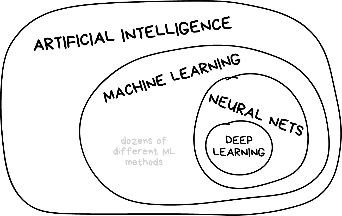
Machine learning is a subset of Artificial Intelligence.
It is a range of methods that learn associations from (training) data.
It then uses these associations for new predictions (i.e., also known as inference).
This ability to do this well is generalising.
These can be useful for a range of problems including:
Prediction problems (e.g., pattern recognition).
Problems that you cannot (or are difficult to) program (e.g., image recognition).
Faster approximations to problems that you can program (e.g., spam classification).
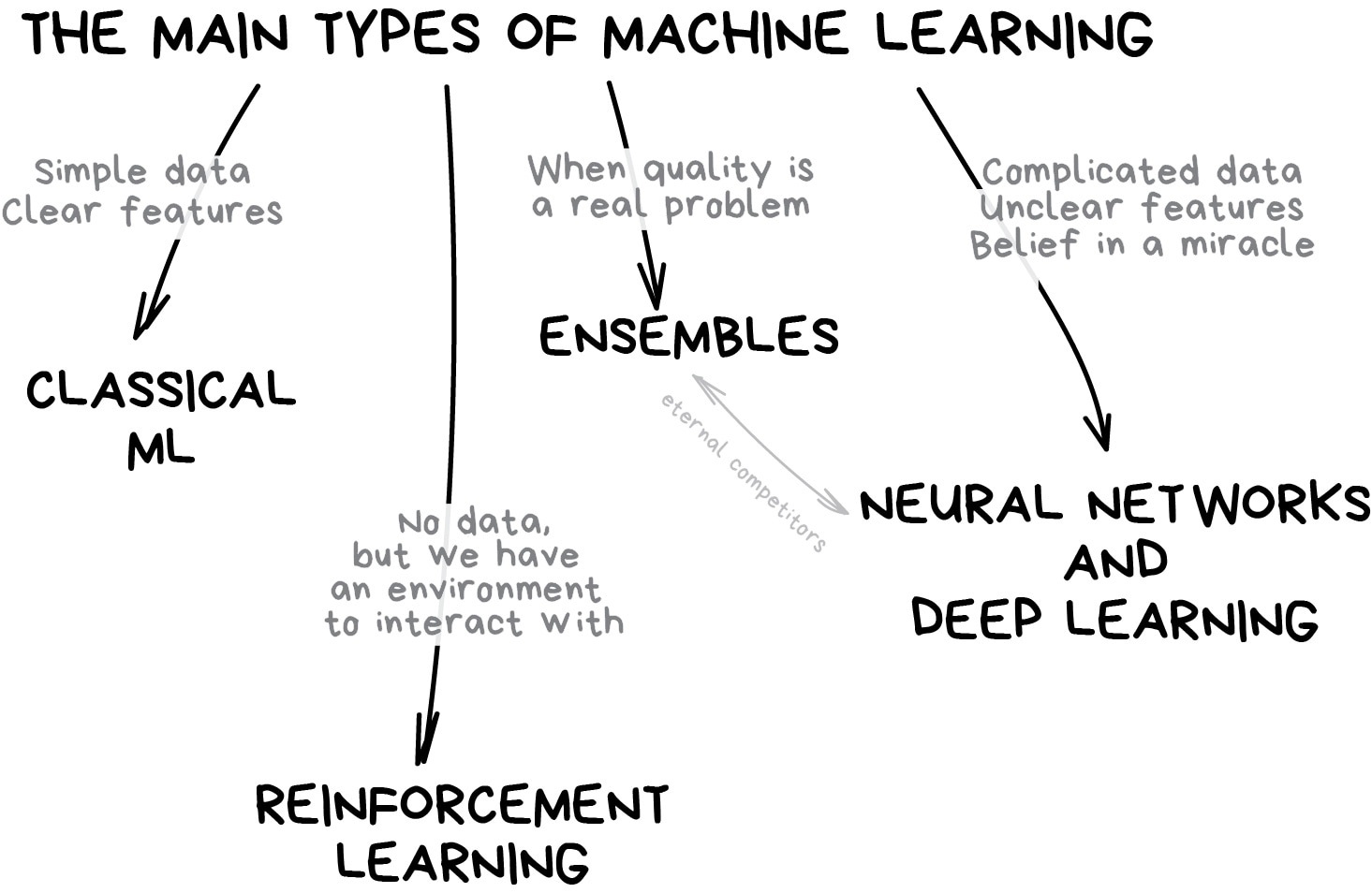
Methods
Within machine learning, there are many different methods.
We’ll focus on classic machine learning and deep learning in this course.
Classic Machine Learning
There are a wide variety of types. Some common ones are:
-
Predict a continuous number using a linear model i.e., fit a straight line.
-
Predict a class of either 0 or 1 i.e., a binary classification problem.
-
Predictions are based on their similarility to their neighbours.
-
Predictions are based their position relative to a decision boundary.
The decision boundary is found by focusing on the two hardest to classify examples and placing support vectors between them.
And many, many more.
Deep Learning (Neural Networks)
Neural networks are models made of layers of neurons.
Neurons (also known as units or nodes) take in inputs and return an output by applying an activation function.
Activation functions (also known as non-linearities) take a weighted sum of inputs from a previous layer, apply a non-linear function, and pass the output onto the next layer.
Common activation functions are:
-
If input is negative, the output equals 0.
If input is positive, the output equals the input.
-
Converts log-odds (we’ll see these later) into probabilities between 0 and 1.
Used for binary classification.
-
Sigmoid for multi-classification.
The neurons are connected in many layers.
Each layer is an input-output transformation.
All the layers together are the model.
The hidden layers between the input layer and output layer are the depth of the model (hence, deep learning).
A common layer is for all the neurons to be fully connected to each other (also known as a dense layer).
The types of layers, how many there are, and how they are connected is the architecture of the neural network.
There are a wide variety of types of neural networks. Some common ones are:
Convolutional Neural Networks (CNN)
A neural network that uses convolutional layers.
These layers find features e.g., for image recognition:
Low-level such as vertical lines, horizontal lines, etc.
Medium-level such as eyes, ears, etc.
High-level such as faces, glasses, etc.
They group operations to reduce the number of parameters learned.
Recurrent Neural Networks (RNN)
For sequential data e.g., time-series, natural language.
Loops over timesteps while maintaining information from previous timesteps.
And many, many more.
Deep learning has been progressing primarily due to scale (bigger datasets and bigger neural networks), investment, and attention (additional research).
Data
The data is a sample of the problem you’re studying.
Data has inputs (also known as features) and outputs (also known as targets).
The inputs are what you provide to the model.
The outputs are what you’re trying to predict.
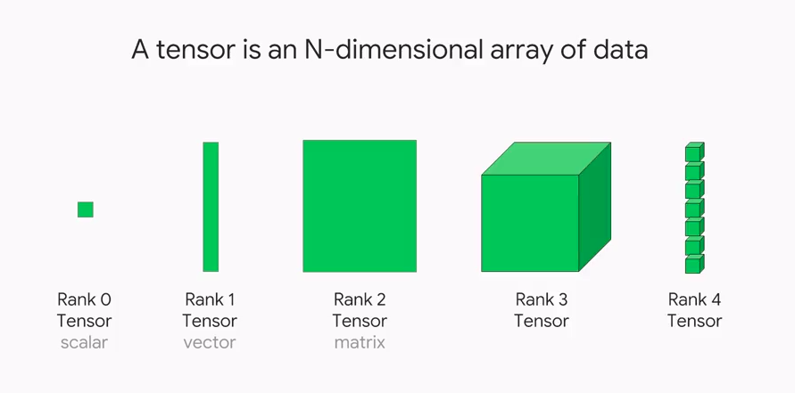
The data is normally in the form of tensors.
Tensors are multi-dimensional arrays:
Scalars are rank-0 tensors.
Vectors are rank-1 tensors.
Matrices are rank-2 tensors.
3+ dimensional arrays are rank-3+ tensors.
Logits and Log-odds
Logits are a vector of raw (non-normalised) predictions from a classification model. For multi-class classification, these are converted to (normalised) probabilities using a softmax function.
Log-odds are the logarithm of the odds of an event. They’re the inverse of the sigmoid function.
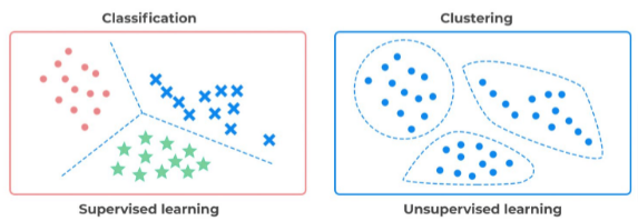
Supervised and Unsupervised
Supervised learning is when you provide labelled outputs to learn from.
Unsupervised learning when you don’t provide any labels.
Below is an example of supervised learning (classify different coloured markers) and unsupervised learning (find clusters within data).
We’ll focus on supervised learning in this course.
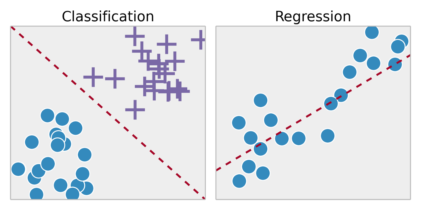
Classification and Regression
Classification problems are those that try to predict a discrete category.
i.e., binary: cat or dog, multi-class: dog breeds (poodle, greyhound, etc.).
Regression problems are those that try to predict a continuous number.
i.e., beans in a jar, house prices.
Below is an example of classification (separate blue circles from purple crosses) and regression (predict a numerical value from the data).
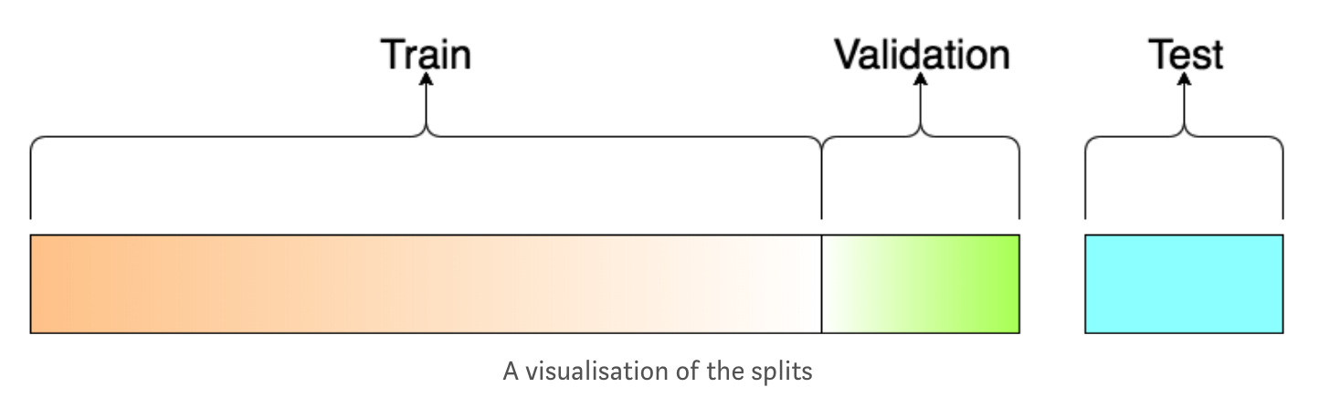
Training, validation, and test splits
The data is normally split into training, validation, and test sets.
The training set is for training the model.
The validation set (optional) is for iteratively optimising the model during training.
The test set is only for testing the model at the end.
This should remain untouched (i.e., held out of training).
Single-use (to ensure representative of future data).
Think of the this like the exam at the end of a course. You don’t want the students to just parrot back the teaching material. You’d like them to demonstrate understanding.
The size of the split depends on the size of the dataset and the signal you’re trying to predict (i.e., the smaller the signal, then the larger the test set needs to be).
For example:
Data set size |
Training split (%) |
Validation split (%) |
Test split (%) |
|---|---|---|---|
Small |
60 |
20 |
20 |
Medium |
80 |
10 |
10 |
Large |
90 |
5 |
5 |
Very large |
98 |
1 |
1 |
The split may benefit from being stratified (preserving original class frequencies) to ensure that each set has a sample of the classes.
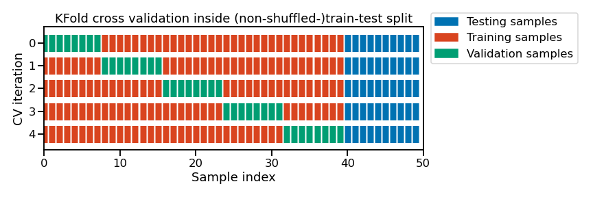
Cross-validation
Cross-validation estimates how well a model generalises to new data before you check it on the single-use test data.
It estimates the variability in the training score.
This repeats the training/validation split multiple times (the test data remains untouched).
There are various methods for cross-validation.
These are mainly variations of K-fold cross-validation, where you split the data up K times (e.g., 5).
Variations then consider stratifying, shuffling, sampling, and replacing.
Below is an example for 5-fold cross-validation (i.e., splitting 5 times).
Hyperparameters
These are what you set before model training.
They control the learning process.
These include, for example:
The number of layers.
The number of units per layer.
The activation function(s).
Whether to use dropout.
The optimiser learning rate.
The batch size.
They are often found through iteratively trying out different options.
This iterative tuning method can be:
Systematically over a grid (i.e., grid-search).
Thorough, but slow. Hence, not suitable for problems with many variables.
Randomly over a grid (i.e., random grid-search).
Faster and more suitable for problems with many variables.
Other options including:
Using Bayes Theorem (i.e., Bayes grid-search) to choose a new set of hyperparameters to test based on the performance of the prior set.
Parameters
These are what the model learns during training (i.e., the weights / biases / coefficients of the model).
The weights first need to be initialised e.g., as zeros, random numbers, etc.
The parameters are then optimised in training.
Model
A model is the machine learning system.
This includes the architechture, parameters, and hyperparameters.
Training
Training is the process of finding the best model.

Loss Function
The loss function measures how accurate the model is during training.
This is measured as the error on single training example.
You always want to minimise the loss function.
A similar concept is the Cost Function, which is the average of the loss functions over the whole training set.
The loss function is a proxy of the metric (covered below) with a smooth gradient. Note, that in some cases it is actually the same as the metric e.g., mean squared error.
Common loss functions are:
-
The average squared loss per example.
-
A measure of the difference between two probability distributions.
Categorical Crossentropy for binary classification.
Sparse Categorical Crossentropy for multi-class classification.
Similar to the Negative Log Loss, except that this takes in log probabilities, instead of raw ones.
Gradient descent
A group of methods to minimise the loss function.
It is how the model gets updated based on the data it sees.
One step of gradient descent includes:
Forward propagate the inputs through the model to calculate the outputs of each neuron.
Calculate the loss (error) and gradient of the loss for these parameters.
Back propagate these gradients back through the model to update the parameters and reduce the loss.
The gradient of the loss is reduced (optimised) in this process (i.e., the gradient descends).
It aims to find the best parameters (i.e., the weights and biases that minimise the loss).
The best parameters represent the single global minimum of the loss (i.e., think of the lowest point in a bowl).
If there are many peaks and valleys in the loss function, then there may be many local minimums (i.e., where the loss function can’t reduce anymore locally).
Common methods of gradient descent are:
Stochastic Gradient Descent (SGD).
Uses 1 training example per iteration.
-
Uses all training examples per iteration.
-
Uses a smaller batch (e.g., 32) of training examples per iteration.
Optimiser
The optimiser is the type of gradient descent used.
A common choice is the Adam (ADAptive with Momentum) optimiser.
Adam combines momentum and RMSprop (Root Mean Squared propagation).
Momentum remembers past gradients to speed up learning and get out of local minimuns.
RMSprop speeds up learning in a specific direction.
Metric
The goal of machine learning is predicting new data.
Hence, the objective is to minimise the test error (as this represents new data).
This is the evaluation metric i.e., the number you primarily care about.
It is helpful to have a single evaluation metric to guide decisions.
Error analysis
This is where you manually analyse the prediction errors from the model to help guide how to improve the model.
An example is a confusion matrix. This is where you aggregate a classifcation model’s correct and incorrect guesses. This is useful to see what classes have more errors.
For example, you could have a classification model to predict whether or not there is a tumor in the image:
Tumor (predicted) |
Non-Tumor (predicted) |
|
|---|---|---|
Tumor (ground truth) |
18 |
1 |
Non-Tumor (ground truth) |
6 |
452 |
So, here there are 19 ground truth images that had tumors (18 + 1), of which the model predicted 18 correct (true positives, TP) and 1 wrong (false negative, FN).
Also, there are 458 ground truth images that did not have tumors (452 + 6), of which the model predicted 452 correct (true negatives, TN) and 6 wrong (false positives, FP).
The precision identifies the frequency of correct predictions for positive cases. Here:
\(precision = TP / (TP + FP)\)
\(precision = 18 / (18 + 6)\)
\(precision = 0.75\)
Recall represents: out of all the possible positive labels, how many did the model correctly identify. Here:
\(recall = TP / (TP + FN)\)
\(recall = 18 / (18 + 1)\)
\(recall = 0.95\)
There is often a trade-off between precision and recall (i.e., one goes up and the other goes down).
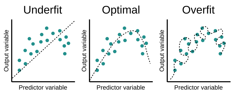
Underfit
A model underfits the data when it has high bias (i.e., systematic errors).
This means the model is too simple to capture the association (i.e., it doesn’t have enough capacity to learn the generalisation).
You can tell that the model underfits because there are both high training errors and high test errors.
To reduce underfitting, try:
Adding more features.
Adding more complex features.
Decreasing regularisation (i.e., decrease the preference for simpler functions).
More training data is unlikely to help a model that underfits the data.
Overfit
A model overfits the data when it has high variance (i.e., varies a lot).
This means the model is too complex to capture the association (i.e., it has too much capacity, so the training data is memorised).
You can tell that the model overfits because there are low training errors but high test errors (i.e., there is a big difference between these errors, where the model doesn’t work well on new data because it overfitted to the noise in the training data).
To reduce overfitting, try:
Adding more data.
Using fewer or simpler features.
Increasing regularisation (i.e., increase the preference for simpler functions).
A smaller neural network with fewer layers/parameters.
Below is an example of underfitting (linear line through non-linear data) and overfitting (very-high order polynomial passing through every training point).
Questions
Question 1
What does deep mean in deep learning?
Question 2
Activation functions help neural networks learn complex functions because they are:
Linear
Non-linear
Question 3
What is a tensor?
Question 4
I have labelled pictures of cats and dogs that I’d like a model to classify.
Is this a supervised or unsupervised problem?
Question 5
I’d like a model to predict house prices from their features.
Is this a classification or regression problem?
Question 6
How many times can I use the test data?
Question 7
I’ve decided on the number of hidden layers to use in my neural network.
Is this a parameter or hyperparameter?
Question 8
Do I want to minimise or maximise the loss?
Question 9
A model underfits the data when it has:
High bias
High variance
Question 10
If my model underfits, what might help:
Adding more features
Adding more data
Question 11
If my model overfits, what might help:
Adding more complex features
Increasing regularlisation
Key Points
Important
Machine learning and deep learning are a range of prediction methods that learn associations from training data.
The objective is for the models to generalise to new data.
They mainly use tensors (multi-dimensional arrays) as inputs.
Problems are mainly either supervised (if you provide labels) or unsupervised (if you don’t provide labels).
Problems are either classification (if you’re trying to predict a discrete category) or regression (if you’re trying to predict a continuous number).
Data is split into training, validation, and test sets.
The models only learn from the training data.
The test set is used only once.
Hyperparameters are set before model training.
Parameters (i.e., the weights and biases) are learnt during model training.
The aim is to minimise the loss function.
The model underfits when it has high bias.
The model overfits when it has high variance.
Further information
Good practices
Start simple.
Incrementally test ideas.
The choice of algortihm depends on the problem/data (i.e., whether you use linear regression, deep learning, etc.).
What assumptions are appropriate?
Future data should be from the same distribution as the training data (to avoid data drift).
The test set should be representative of the future data you’re trying to predict. For example:
For time series, test data may be 2021, while training data was 2015-2020.
For medical application, test data may be completely new patients, not multiple visits from same patients in training data.
Consider ways to reduce the dimensionality of the data (e.g., using PCA, Principle Component Analysis).
Have a baseline to compare the model skill against (i.e., simple model, human performance, etc.).
Caveats
Predictions are primarily based on associations, not explanations or causation.
Predictions and models are specific to the data they were trained on.
Resources
Bold are highly-recommended.
Hands-On Machine Learning with Scikit-Learn, Keras, and TensorFlow, 2nd Edition, Aurélien Géron, 2019, O’Reilly Media, Inc.
Deep Learning with Python, 2nd Edition, François Chollet, 2021, Manning.
Artificial Intelligence: A Modern Approach, 4th edition, Stuart Russell and Peter Norvig, 2021, Pearson.
Machine Learning Yearning, Andrew Ng.
Online courses
Bold are highly-recommended.
Machine learning
Machine learning, Coursera, Andrew Ng.
CS229, Stanford University: Video lectures.
Machine Learning for Intelligent Systems, Kilian Weinberger, 2018.
CS4780, Cornell: Video lectures.
Artificial Intelligence: Principles and Techniques, Percy Liang and Dorsa Sadigh, CS221, Standord, 2019.
Machine learning in Python with scikit-learn, scikit-learn developers, 2022.
Deep learning
Deep Learning Specialization, Coursera, DeepLearning.AI (NumPy, Keras, TensorFlow)
CS230, Stanford University: Video lectures, Syllabus
NYU Deep Learning, Yann LeCun and Alfredo Canziani, NYU, 2021 (PyTorch)